Hi everybody.
May be you know, or used long ago, the Gantt chart. This is a visual simple organiser. Anybody can build such chart manually in MS Excel. But I know that building of this chart can be very easy by Excel's feature as Conditional Formatting.
I show you simple example from Dave Bruns.
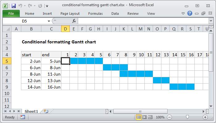
So you have some data with Starting dates and Finishing dates, from 2th of June to 16th of June. Ok. These dates are placed in two columns B and C our table. In 4th row of table we place all range of dates with Custom format: 1-st of June as 1 2nd of June as 2 and so on. Until 17th of June.

Generic formula for each cell is
=AND(date>=start,date<=end)
To build a Gantt chart, you can use Conditional Formatting with a formula based on the AND function.
In the example shown, the formula applied to D5 is:
=AND(D$4>=$B5,D$4<=$C5)
=AND(D$4>=$B5,D$4<=$C5)
How this formula works?
The trick with this approach is the calendar header, which is just a series of valid dates, formatted with the custom number format "d". This makes it easy to set up a conditional formatting rule that compares the date associated with each column with the dates in columns B and C.
The formula is based on the AND function, configured with two conditions. The first conditions checks to see if the column date is greater than or equal to the start date:
D$4>=$B5
D$4>=$B5
The second condition checks that the column date is less than or equal to the end date:
D$4<=$C5
D$4<=$C5
When both conditions return true, the formula returns TRUE, triggering the blue fill for the cells in the calendar grid.
Note: both conditions use mixed references to ensure that the references update correctly as conditional formatting is applied to the calendar grid.
It's easy.

No comments:
Post a Comment
А что вы думаете по этому поводу?